Mathematics of the AHP
You don't need to understand the mathematics behind the AHP to use it effectively. You just need to understand the basic concepts like pairwise comparisons, the 1–9 scale, and what a good consistency ratio looks like. If that's all you are interested in, head on over to our Introduction to the AHP article. On the other hand, once you master the basics you might want to peek behind the curtain to see what calculations are performed to produce the outputs. This article aims to describe the whole process, starting from high-school level concepts such as vectors and matrices. This should prepare you for the more advanced topics, such as the eigenvector calculation used to produce the priority weights. Towards the end, there is a complete worked decision, followed by the sensitivity analysis that tests how firmly it stands.
The literature contains several ways to derive priorities from a comparison matrix, and several consistency indices. They agree on consistent matrices and differ slightly on inconsistent ones. This article describes the standard approach, the one the decisionpoint.io app uses: Saaty's eigenvector method and consistency ratio, plus the two extensions most implementations need (Harker's method for missing comparisons and the geometric mean for groups). If you want to learn more about the alternatives, Brunelli (2015) provides a good introduction.
How to read the notation
To begin, let's take a tour of the notation that we will be using. The table is worth glancing through now, but there is no need to memorise it as every symbol will be explained when it first appears.
| Symbol | How to read it |
|---|---|
| A matrix: a grid of numbers. Written as a bold capital letter. | |
| The entry of in row , column . In the AHP it holds the judgment comparing element with element . | |
| , | A vector: a list of numbers, written as a bold lower-case letter. is its th entry. In the AHP, is the priority vector: the weights. |
| Transpose: the vector or matrix turned on its side, so a row becomes a column and a column becomes a row. Explained below. | |
| The vector of ones, . Saaty's books write it as ; Brunelli and this article write . | |
| The largest eigenvalue of a matrix (lambda). Defined in the eigenvector section. | |
| The number of elements being compared. | |
| The number of participants in a group decision. | |
| , | Sum and product over an index. means ; is the same with multiplication. |
| CI, RI, CR | Consistency index, random index, consistency ratio. Defined in the consistency section. |
What are vectors and matrices?
Let's start with an easy one: a vector is simply a list of numbers, nothing more. For example, the priorities of three criteria can be grouped together to form a vector with three entries:
A matrix is a grid of numbers with rows and columns. The entry in row , column is written , row first, column second, so is the entry in row 2, column 3. It is the same idea as a spreadsheet naming a cell, except both coordinates are numbers and the row comes first.
The transpose is a piece of notation that often appears in AHP publications, and can trip you up if you haven't come across it before. A vector's numbers can be laid out across the page, as a row vector, or down the page, as a column vector. On its own the layout means nothing: it's the same vector either way. It starts to matter when you need to multiply a matrix and a vector, because then you have to be explicit about which layout you mean; the two choices pair the entries with the matrix differently. The standard choice, always used for the AHP, is to treat the vector as a column. But vectors are often written across the page by default, because a row fits in a sentence. The transpose, indicated by a superscript , simply means that this row vector should be turned on its side and treated as a column.
Nothing about the numbers changes; the transpose is bookkeeping, not calculation. So, when an AHP paper writes , read it as: these are the entries of , and is a column.
How do you multiply vectors and matrices?
Next, let's look at some building blocks that we will need later on. The first is very simple: to multiply a vector by a single number (a scalar) multiply every entry in the vector by the scalar.
There are two ways to multiply vectors: the dot product and the cross product. We won't need the cross product, so we'll ignore that one. The dot product of two vectors multiplies the corresponding entries and adds the results.
Matrix-times-vector is one dot product per row: row of the result is row of the matrix dotted with the vector. This is where column shape becomes important. Each row of the matrix reads across, the vector beside it reads down, and the matching entries pair up:
The animation below walks through the same example one row at a time.
Multiplying a matrix by a matrix repeats this for each column of the second matrix, but again we won't need that so we'll ignore it. For AHP calculation we only need matrix-times-vector, the dot product, and scalar multiplication.
What is an eigenvector?
The easiest way to understand eigenvectors is to look at vectors the way physicists do. So far we have treated a vector as a list of numbers, but a list like can also be drawn as an arrow: go 3 across and 1 up. The same numbers describe both a direction and a length, which is why physics uses vectors for forces and velocities. A vector with 2 entries can represent a 2D arrow, and a vector with 3 entries a 3D arrow. It gets harder to visualise in higher dimensions, but the concept is the same: we can think of vectors as both lists of numbers and arrows with a particular length and direction.
Multiplying a matrix by a vector, seen as an arrow, produces a new arrow. In most cases the new arrow points in a different direction, and is longer or shorter. But for some combinations of matrices and vectors, the arrow keeps pointing in the same direction, and only the length changes. These vectors are the eigenvectors of the matrix, and the stretch factor (lambda) is the eigenvalue paired with each one. Multiplying the vector by the eigenvalue gives the same result as multiplying the vector by the matrix:
Here is a 2×2 example: an AHP comparison matrix with one judgment, saying that the first element is twice as important as the second.
The vector comes out as itself times 2, so it is an eigenvector with eigenvalue 2. Scaled to sum to 1 it reads : weights of 67% and 33%, exactly what a "twice as important" judgment should produce. An × matrix has up to eigenvalues, with the largest one written .
There is a guarantee behind all of this: the Perron–Frobenius theorem, which says that a matrix whose entries are all positive has a single largest eigenvalue, and that the corresponding eigenvector has positive entries. Comparison matrices are all positive, so this principal eigenvector always exists, is unique once scaled to sum to 1, and never contains a zero or negative weight. That is why the AHP calculation always gives a well-defined answer for any set of judgments.
What is a pairwise comparison matrix?
A pairwise comparison matrix collects judgments about elements. Entry tells us how many times more important element is than element . Judgments use the 1–9 Saaty scale. Two rules follow from what the judgments mean. Every element is equal to itself, and if is 3 times , then is a third of :
At first glance the matrix seems to require judgments. However, if we look closer, we see that the diagonal is always 1, and the lower half is a mirror image of the upper half. That leaves real judgments: 3 for 3 elements, 10 for 5, 45 for 10.
Here is the sample matrix from our Introduction to the AHP, which weights three smartphone criteria, with Camera judged 3 times as important as Price, Camera 5 times Battery, and Price 3 times Battery.
Imagine if we had perfect knowledge of the true weights for a decision. Every judgment would be an exact ratio of weights, , and the whole matrix would be:
A matrix of this form is called consistent. Perfect consistency like this rarely happens in the real world, but the AHP calculation is built to cope with that. Take a mental note of this ideal form, as the next section is built on it.
Why does the eigenvector give the weights?
Before the derivation, it is worth asking why the AHP reaches for an eigenvector at all, rather than simply averaging the judgments in each row. The answer is inconsistency. When the judgments contradict each other, an average quietly ignores the contradictions, while the eigenvector redistributes them across all the weights at once, so that the result is the single set of weights the whole matrix best agrees with. That is the method's central claim, and the rest of this section shows where it comes from.
Take the consistent matrix above and multiply it by its own weight vector. Row gives:
Each term collapses: . So : for a consistent matrix, the true weight vector is an eigenvector, and its eigenvalue is exactly . The weights are not merely related to the matrix; they are sitting inside it, recoverable by an eigenvector calculation.
Saaty's key insight (1977) was to extend this to real, imperfect matrices: keep the same equation, with the largest eigenvalue in place of . The priority vector is defined as the solution of
The first equation is a matrix times a column vector, exactly as in the previous section, so no transpose is needed. The second condition scales the weights to sum to 1, since an eigenvector times any number is still an eigenvector. Here the transpose works in the opposite direction: is a column, and turns it on its side into a row. A row times a column is a single dot product, just like one row of a matrix-times-vector calculation. Dotting with the vector of ones simply adds up the entries:
Without the transpose, and would be two columns side by side, which isn't a valid product. The Perron–Frobenius theorem guarantees this exists, is positive, and is unique. For a consistent matrix and the method returns the exact weights; for a slightly inconsistent one it returns a compromise that tolerates the contradictions, and rises above by an amount that measures them. That excess is the basis of the consistency check.
How is the eigenvector computed? The power method
Unfortunately, there isn't a simple formula where we can plug in a matrix and get the principal eigenvector. Instead, we use an iterative process that converges on the answer through repeated steps. The standard technique, used by decisionpoint.io, is the power method. It works as follows: any starting vector can be thought of as a blend of the matrix's eigenvectors, and each multiplication by stretches the principal one more than the rest, because it has the largest eigenvalue. So with every round its share of the blend grows, and after a few rounds the other components are too small to see: the vector settles onto the principal eigenvector and stops moving. Here is the algorithm:
- Start with , meaning no opinion yet: every element equal.
- Multiply: .
- Normalise: divide every entry of by the sum of its entries, so they sum to 1.
- Compare with the previous vector. If the squared distance between them (sum of squared differences) is below , stop. Otherwise repeat from step 2, up to a cap of 12 iterations.
On the smartphone criteria matrix, the method converges in five iterations:
| Iteration | Sum | After normalising | Squared distance | |
|---|---|---|---|---|
| 1 | (9, 4.333, 1.533) | 14.867 | (0.6054, 0.2915, 0.1031) | 1.46 |
| 2 | (1.9955, 0.8027, 0.3214) | 3.1196 | (0.6397, 0.2573, 0.1030) | 0.0023 |
| 3 | (1.9267, 0.7796, 0.3167) | 3.0230 | (0.6373, 0.2579, 0.1048) | 8.8 × 10⁻⁶ |
| 4 | (1.9349, 0.7846, 0.3182) | 3.0377 | (0.6369, 0.2583, 0.1048) | 3.3 × 10⁻⁷ |
| 5 | (1.9356, 0.7849, 0.3182) | 3.0387 | (0.6370, 0.2583, 0.1047) | 1.9 × 10⁻⁹ |
The weights are : Camera 63.7%, Price 25.8%, Battery 10.5%. Watch the Sum column. Once is nearly the eigenvector, , and since sums to 1, the sum of drifts toward itself: 3.0387 by iteration 5.
The sum above gives us an estimate of , but once we have the principal eigenvector we can get a more precise value using a formula called the Rayleigh quotient. At convergence . Taking the dot product of each side with turns both sides into ordinary numbers: . Dividing both sides by the number leaves by itself:
The stopping threshold of on the squared distance, and the cap of 12 iterations, follow Goepel's analysis of numerical accuracy in AHP calculations. In practice five or six iterations give weights stable to four decimal places, far more precision than needed in most circumstances.
A hand method for checking
A quicker estimate needs no iteration: divide each column by its sum, then average each row. For the criteria matrix, the column sums are (1.533, 4.333, 9). Dividing and averaging gives (0.633, 0.261, 0.106), against the exact (0.637, 0.258, 0.105). The estimate is close because the matrix is nearly consistent, and it is exact whenever the matrix is fully consistent.
This column-normalisation method is sometimes mistaken for the AHP calculation itself, because it appears in so many tutorials and spreadsheets. It is not. Saaty (1980) presents it as one of several hand approximations to the eigenvector, which has been the definition of the priorities since his first paper in 1977. Treat it as a sanity check on an implementation, not as a substitute for the power method.
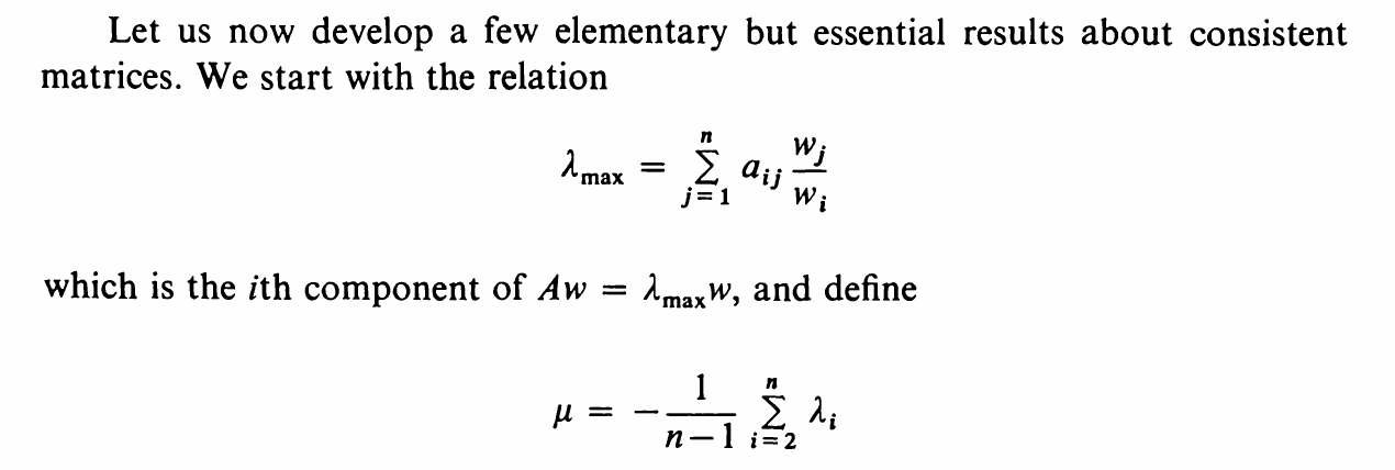
The same kind of check exists for . The Rayleigh quotient above is the least-squares estimate: the value of that makes and as close as possible. The hand-friendly alternative is the one in the excerpt from Saaty's book at the top of this page: divide each entry of by the matching entry of , which gives separate estimates of , and average them. For an exact eigenvector every estimate agrees; for an approximation the two formulas differ only in how they average out the residual error, and both give 3.0385 for the criteria matrix.
How is consistency measured?
Judgments can contradict each other. If Camera is 3 times Price and Price is 3 times Battery, then Camera should be 3 × 3 = 9 times Battery. The judge entered 5. Each such triple of judgments is called a triad, and perfect consistency means every triad obeys the rule:
Nobody meets that standard, and the AHP does not expect them to. Instead, it measures how far the judgments fall short, using a fact about eigenvalues: for a positive reciprocal matrix, always, with equality only when the matrix is consistent (Saaty 1977). The excess of over , spread over the matrix size, is the consistency index:
CI alone is hard to interpret, because larger matrices pick up more inconsistency by chance. Saaty's answer was to calibrate against randomness itself: generate many random reciprocal matrices of size , average their CI, and call the result the random index . The consistency ratio compares your matrix against that baseline:
| 3 | 4 | 5 | 6 | 7 | 8 | 9 | 10 | 11 | 12 | 13 | 14 | 15 | |
| 0.58 | 0.90 | 1.12 | 1.24 | 1.32 | 1.41 | 1.45 | 1.49 | 1.51 | 1.48 | 1.56 | 1.57 | 1.59 |
These are Saaty's values, and they are what decisionpoint.io uses. The first eight are the classic table; the entries for 11 to 15 come from Saaty's later publications, and decisionpoint.io allows at most 15 elements in any one comparison set, so the table always covers the matrix at hand. The dip from 1.51 at = 11 to 1.48 at = 12 is in Saaty's published table; Donegan and Dodd (1991) trace it to a change in the number of random matrices sampled. RI is a simulation estimate, so published tables differ slightly: Brunelli's book, for example, tabulates Alonso and Lamata's estimates (0.5245 for = 3 against Saaty's 0.58). The differences move a CR by a few percent at most, but when two AHP tools disagree in the second decimal place of a CR, a different RI table is the usual reason.
The working rule, due to Saaty, is to accept the judgments when , and revisit them when it is higher. A CR of 0.1 means the judgments are 10% as inconsistent as random noise. For the smartphone criteria matrix: , so CI = (3.0385 − 3) / 2 = 0.0193 and CR = 0.0193 / 0.58 = 0.033, which sits comfortably inside the threshold. When a matrix fails the check, decisionpoint.io can point at the problematic judgment triads and ask the user how they want to rework the judgments to make them more consistent.
The threshold is a convention about how much contradiction to tolerate, not a mathematical boundary, and it has been argued in both directions. Saaty himself suggested tighter limits for the smallest matrices, 0.05 for = 3 and 0.08 for = 4, on the grounds that random inconsistency is harder to come by with so few judgments. Goepel, whose AHP template and AHP-OS tool are widely used, argues from the other side: across corporate projects with about 80 participants he found a median CR of 0.16 on the 1–9 scale, so the 10% rule would have rejected most questionnaires. His template documentation recommends an acceptance threshold between 0.1 and 0.2, and in one project he accepted up to 0.3 (Goepel 2013). His tools also compute CR from Alonso and Lamata's linear fit to the random index rather than from a table,
which tracks Saaty's values closely for of 4 or more, extends beyond the end of any table, and gives 0.040 instead of 0.033 for the smartphone matrix (Goepel 2018). decisionpoint.io applies the 0.1 rule with Saaty's table at every size, which remains the common practice. Treat the stricter small-matrix limits and the looser survey-based practice as context for reading a borderline CR, not as alternative rules.
An implementation note: in floating-point arithmetic, for a perfectly consistent matrix can come out slightly below , such as 2.9999999. Implementations clamp CI to zero in that case rather than report a negative value.
What happens when comparisons are missing?
Real decision makers skip comparisons. They run out of time, or cannot compare two unlike things with any confidence. The eigenvector method as described needs every entry, so a method of repairing incomplete matrices is required. The standard one is Harker's method (1987), which builds an auxiliary matrix :
where counts the missing entries in row . Each missing judgment becomes a zero, and the diagonal entry of its row goes up by one. Then compute the eigenvector of the same way as before.
The trick might not be obvious until you see what the diagonal bump does. A missing entry should ideally hold , and in the product that entry would contribute . Adding 1 to the diagonal contributes the same . So acts on the weight vector as if every missing judgment had been filled in perfectly consistently with the answer.
A worked example
Three elements, two judgments given, the 1–3 comparison skipped (dots mark the missing pair):
Rows 1 and 3 each lost one entry, so their diagonals rise from 1 to 2. The principal eigenvector of is , and you can verify it yourself with one multiplication:
The weights make sense: the given judgments say element 1 is twice element 2, and element 2 twice element 3, so the method fills the gap with the implied 4-to-1 ratio. Here and CI = 0. That is no accident. Consistency can only be measured where judgments overlap, and with just comparisons there is no overlap to contradict. Which is also the floor: at least comparisons, forming a chain that connects every element, are needed before any weights can be computed at all. decisionpoint.io tracks this and reports which comparisons are missing and whether the set is connected.
How are group judgments combined?
When people each judge the same pair, the group value is the geometric mean of their judgments, calculated by multiplying them together and taking the th root. Applied entry by entry, it merges comparison matrices into one group matrix, which then goes through the same calculation as a regular comparison matrix:
where is participant 's judgment on the pair. Two people judging 3 and 6 combine to .
Why the geometric mean rather than the familiar arithmetic one? Because the merged matrix still has to be a valid comparison matrix, which means every mirror pair of entries must stay reciprocals of each other. The arithmetic mean breaks that rule, while the geometric mean obeys it. Suppose two people take opposite views: one says 3, the other 1/3. The geometric mean gives , a balanced group. The arithmetic mean gives (3 + 1/3) / 2 = 1.67, and averaging the mirror entries below the diagonal also gives 1.67. But a comparison matrix needs the mirror entry to be the reciprocal, 1/1.67 = 0.6, so the aggregated matrix is no longer a valid comparison matrix at all. Aczél and Saaty (1983) proved that the geometric mean is the only aggregation rule satisfying their natural conditions: unanimity (if every participant gives the same judgment, the group judgment is that value) and the reciprocal property (aggregating everyone's reciprocal judgments gives the reciprocal of the aggregate), along with mild regularity requirements such as treating participants symmetrically. Forman and Peniwati (1998) call this approach aggregation of individual judgments (AIJ); the alternative, computing each person's weights first and averaging those (AIP), suits groups that do not share one model of the decision. decisionpoint.io uses AIJ with equal participant weights, as described in the group AHP announcement.
A small implementation detail: decisionpoint.io stores every judgment as a fraction, so "Battery is 3 times Camera" on Camera's row is 1/3 exactly, not 0.3333…. The geometric mean is computed as the geometric mean of the numerators over the geometric mean of the denominators, which is the same number with less floating-point drift, and it keeps aggregated reciprocal pairs exact mirror images of each other.
How do weights turn into final scores?
A full AHP decision produces one comparison matrix for the criteria and one matrix of alternatives per criterion. The criteria matrix yields the criteria weights ; each per-criterion matrix yields local priorities , how well alternative does on criterion . The final score is a weighted sum:
This is the distributive mode of synthesis, in which each criterion's local priorities sum to 1, and it is what decisionpoint.io uses. The literature also has an ideal mode, which instead divides each criterion's local priorities by the largest of them, so the best alternative on every criterion scores 1. The two modes usually agree on the ranking. They differ in rank reversal: under the distributive mode, adding or removing an alternative can reorder the others, which Belton and Gear (1983) raised as an objection and the ideal mode was introduced to address. Saaty's position is that the distributive mode is right when alternatives compete for a share of something, and the ideal mode when only the single best alternative matters.
With subcriteria, weights multiply down the tree. If Cost carries 0.6 of the decision and splits into Purchase price at 0.7 and Running cost at 0.3, their global weights are 0.6 × 0.7 = 0.42 and 0.6 × 0.3 = 0.18. The synthesis then sums over the leaf criteria only, each with its global weight. Every level is normalised to sum to 1, so the final scores do too.
The synthesis step is also where a decision can stop early. A criteria-only analysis ends with the weights themselves, for problems where the weights are the deliverable, such as budget shares, scoring rubrics, and KPI weighting.
A complete worked example
This section applies everything above to one decision, end to end: choose a smartphone from X, Y and Z, using Camera, Price and Battery. Twelve judgments in total: 3 for the criteria, 9 for the alternatives.
The criteria matrix and its results, from the power method section:
The alternatives are compared three times, once per criterion. Each 3×3 matrix goes through the same power method. All three happen to share one structure (the judgments are permutations of 1/5, 1/3 and 2), so each has and CR = 0.003:
| With respect to | X vs Y | X vs Z | Y vs Z | Local priorities (X, Y, Z) |
|---|---|---|---|---|
| Camera | 1/5 | 1/3 | 2 | 0.109, 0.582, 0.309 |
| Price | 5 | 2 | 1/3 | 0.582, 0.109, 0.309 |
| Battery | 3 | 1/2 | 1/5 | 0.309, 0.109, 0.582 |
Synthesis is one weighted sum per phone. For Phone Y: 0.637 × 0.582 + 0.258 × 0.109 + 0.105 × 0.109 = 0.410.
| Criterion (weight) | Phone X | Phone Y | Phone Z |
|---|---|---|---|
| Camera (0.637) | 0.109 | 0.582 | 0.309 |
| Price (0.258) | 0.582 | 0.109 | 0.309 |
| Battery (0.105) | 0.309 | 0.109 | 0.582 |
| Final score | 0.252 | 0.410 | 0.338 |
Phone Y wins on the strength of its camera under the most important criterion. These are the same numbers shown in Introduction to the AHP; now you can see how they were derived. To see the pipeline run on a larger decision, open the worked AHP example: family car selection in decisionpoint.io.
How is sensitivity analysis computed?
The final scores depend on the criteria weights, and the weights came from human judgments. Sensitivity analysis asks how much the result would change if one of those weights were different. Pick a criterion and give its weight a new value between 0 and 1. The other criteria must still account for the rest of the decision, so their weights are rescaled proportionally: each keeps the share of the remainder it had before.
Substituting these into the synthesis formula gives each alternative's score as a function of :
Everything in that expression except is a constant, so each alternative's score is a straight line in . At the criterion is switched off, and at it is the only criterion, where the score is just the local priority . The sensitivity chart in decisionpoint.io is exactly this picture: one line per alternative, with the current weight marked, and the current scores where the lines meet that mark. A tipping point is a weight at which two lines cross and the alternatives swap places. Because the lines are straight, two scores evaluated at the ends of the range fix each line completely, and the crossing of alternatives and can be solved exactly rather than searched for by stepping through weights:
A crossing only counts if falls strictly inside the range; two lines that meet only at an endpoint, or that coincide throughout, do not swap anything.
Rating stability
Tipping points are plentiful on any real decision, so the Stability Overview in decisionpoint.io reduces them to one number per criterion, following Triantaphyllou and Sánchez (1997). Their analysis shows that a sensitivity measure must make two choices: whether to count any swap of positions or only a change of winner, and whether to measure the change to a weight in absolute points or relative to the weight itself. The measure they call Percent-Top takes the second option both times. For criterion , find the nearest crossing in either direction at which some other alternative overtakes the current leader, and report it relative to the current weight:
Swaps further down the ranking are ignored, and a two-point change counts for more on a weight of 4% than on a weight of 50%. decisionpoint.io labels as sensitive, 10% to 25% as moderate, and anything larger as stable; a criterion with no such crossing in either direction can never change the winner and is stable too. The bands are our convention, as the paper leaves labelling to the reader. For a subcriterion, the weight is varied within its own group while the parent's weight stays fixed, so the relative change in its local weight equals the relative change in its global weight, and top-level criteria and subcriteria read on the same scale. The stability analysis announcement shows the measure applied to a ten-criterion decision.
The smartphone example
Take Camera, the heaviest criterion at 0.637. Setting rescales Price and Battery to 0.712 and 0.288; setting leaves only the Camera priorities. Evaluating the three scores at each end gives the lines:
| Phone | Score at | Score at | Score at |
|---|---|---|---|
| X | 0.503 | 0.109 | 0.252 |
| Y | 0.109 | 0.582 | 0.410 |
| Z | 0.388 | 0.309 | 0.338 |
Phone Y's line is the only one rising, so increasing the Camera weight can never unseat it. Decreasing it, Y first meets Z: = 0.109 − 0.388 = −0.279 and = 0.582 − 0.309 = 0.273, so the crossing is at = −0.279 / (−0.279 − 0.273) = 0.505. That is a relative change of (0.505 − 0.637) / 0.637 = −20.7%: if Camera matters about a fifth less than the judgments say, Phone Z wins instead, and Camera is rated moderate. Running the same calculation for the other two criteria, Price would have to rise from 0.258 to 0.444 (+72%) before Phone X overtakes Y, and Battery from 0.105 to 0.224 (+114%) before Z does, so both are stable. The decision rests mainly on how much the camera really matters, which is a useful thing to know before acting on it.
Quick reference
A recap of key concepts that we encountered above.
| Name | Formula | Meaning |
|---|---|---|
| Reciprocity | Each pair needs one judgment; the diagonal is 1. | |
| Consistency condition | Every indirect path agrees with the direct judgment. | |
| Priority vector | Weights are the principal eigenvector, scaled to sum to 1. | |
| Power method step | Multiply and normalise until the change is below . | |
| Rayleigh quotient | Estimates the largest eigenvalue from the eigenvector. | |
| Consistency index | Zero when consistent; grows with contradiction. | |
| Consistency ratio | CI against random baseline; accept at . | |
| Harker fill | , missing | Handles missing comparisons; then proceed as normal. |
| Group aggregation | Geometric mean of the participants' judgments, per pair. | |
| Synthesis | Final score: local priorities weighted by criteria weights. | |
| Sensitivity line | Score as criterion 's weight varies; straight in , so crossings solve exactly. | |
| Percent-Top stability | Nearest relative weight change that changes the winner; sensitive below 10%, moderate to 25%, else stable. |
References
Most of these papers are annotated, with verified links and notes on what each contributed, in the AHP Library.
Aczél, J. & Saaty, T.L. (1983). "Procedures for synthesizing ratio judgements." Journal of Mathematical Psychology, 27(1), 93-102.
Alonso, J.A. & Lamata, M.T. (2006). "Consistency in the analytic hierarchy process: a new approach." International Journal of Uncertainty, Fuzziness and Knowledge-Based Systems, 14(4), 445-459.
Belton, V. & Gear, T. (1983). "On a short-coming of Saaty's method of analytic hierarchies." Omega, 11(3), 228-230.
Brunelli, M. (2015). Introduction to the Analytic Hierarchy Process. SpringerBriefs in Operations Research. doi:10.1007/978-3-319-12502-2. Open-access postprint at Aaltodoc.
Donegan, H.A. & Dodd, F.J. (1991). "A note on Saaty's random indexes." Mathematical and Computer Modelling, 15(10), 135-137.
Forman, E. & Peniwati, K. (1998). "Aggregating individual judgments and priorities with the Analytic Hierarchy Process." European Journal of Operational Research, 108(1), 165-169.
Goepel, K.D. (2013). "Implementing the Analytic Hierarchy Process as a standard method for multi-criteria decision making in corporate enterprises: a new AHP Excel template with multiple inputs." Proceedings of the International Symposium on the Analytic Hierarchy Process, Kuala Lumpur. bpmsg.com.
Goepel, K.D. (2018). "Implementation of an online software tool for the Analytic Hierarchy Process (AHP-OS)." International Journal of the Analytic Hierarchy Process, 10(3), 469-487. doi:10.13033/ijahp.v10i3.590.
Goepel, K.D. (2013). "AHP Excel template numerical accuracy." bpmsg.com.
Harker, P.T. (1987). "Incomplete pairwise comparisons in the analytic hierarchy process." Mathematical Modelling, 9(11), 837-848.
Hefferon, J. Linear Algebra. Free textbook, for readers who want the matrix material in full. hefferon.net/linearalgebra.
Saaty, T.L. (1977). "A scaling method for priorities in hierarchical structures." Journal of Mathematical Psychology, 15(3), 234-281.
Saaty, T.L. (1980). The Analytic Hierarchy Process. McGraw-Hill. Chapter 7 covers positive reciprocal matrices, the computation of the eigenvector (§7-4) and consistency (§7-5).
Saaty, T.L. (2008). "Decision making with the analytic hierarchy process." International Journal of Services Sciences, 1(1), 83-98.
Triantaphyllou, E. & Sánchez, A. (1997). "A sensitivity analysis approach for some deterministic multi-criteria decision-making methods." Decision Sciences, 28(1), 151-194. doi:10.1111/j.1540-5915.1997.tb01306.x.